Systèmes mécaniques oscillants

Systèmes oscillants

Un système mécanique oscillant est un système dont le centre d'inertie G décrit un mouvement périodique de va-et-vient autour d'une position d'équilibre stable (ex : balancier d'une horloge, membrane d'un haut-parleur, balançoire...).

pendule simple

pendule de torsion

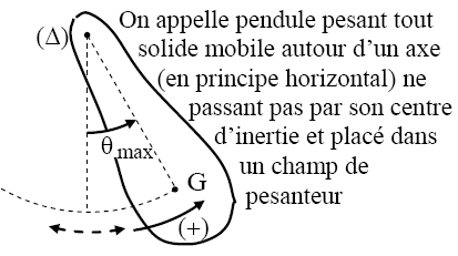
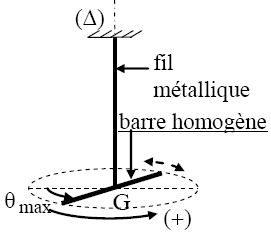
pendule pesant

pendule élastique

 

Le pendule simple est une modélisation du pendule pesant.

Équilibre stable : état dans lequel un corps écarté de sa position d'équilibre tend à y revenir

Un oscillateur mécanique est dit libre quand, une fois écarté de sa position d'équilibre, il est abandonné à lui-même.

La période propre d'un oscillateur libre non amorti est la durée entre deux passages consécutifs de l'oscillateur par la même position et dans le même sens.

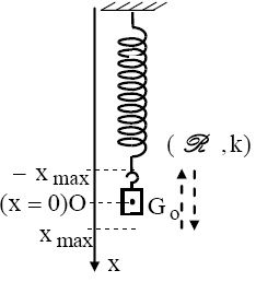
Étude du dispositif solide-ressort (pendule élastique)

Étude expérimentale

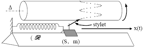
cylindre en rotation uniforme autour de son axe $\Delta$

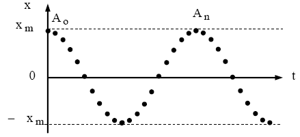
Écartons le cavalier (S) de sa position d'équilibre stable $(\mathrm{O})$ d'une distance $d$ et lâchons-le, à $\mathrm{t}=0$, sans vitesse initiale. Il effectue des oscillations libres autour de $(\mathrm{O})$.

Enregistrons, pendant des durées égales $\tau=40 \mathrm{~ms}$, les positions successives de (S) : le mouvement de (S) se reproduit identique à lui-même : il est périodique de période $\mathrm{T}_{\mathrm{o}} \cdot\left(\mathrm{T}_{\mathrm{o}}=\mathrm{n} \cdot \tau=20 \times 40=800 \mathrm{~ms}=0,8 \mathrm{~s}\right)$
$(\mathrm{n}+1)$ : nombre de positions enregistrées depuis $\mathrm{A}_{\mathrm{o}}$ jusqu'à $\mathrm{A}_{\mathrm{n}}$.

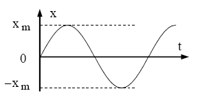
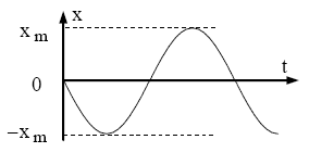
L'enregistrement montre que la fonction $\mathrm{x}=\mathrm{f}(\mathrm{t})$ est sinusoïdale, $\left(-\mathrm{x}_{\max } \leq \mathrm{x} \leq \mathrm{x}_{\max }=\mathrm{d}\right)$.

Étude dynamique

Équation différentielle

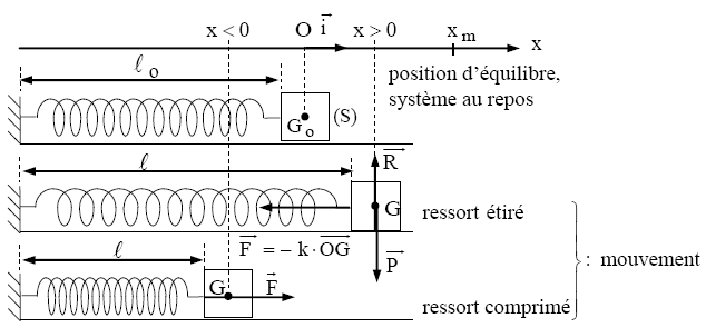
• Système étudié : le solide.
• Référentiel : terrestre (galiléen par approximation).
• Forces extérieures : $\overrightarrow{\mathrm{P}}$ : poids du solide.

                                               $\overrightarrow{\mathrm{R}}$ : la réaction du support.         

                                               $\overrightarrow{\mathrm{F}}$ : la tension du ressort.

La force $\overrightarrow{\mathrm{F}}$ agit sur le solide de manière à le ramener vers sa position d'équilibre lorsqu'il s'en écarte : c'est une force de rappel.

Quelque soit l'orientation de l'axe $\mathrm{Ox}$ et que le ressort soit étiré (allongé) ou comprimé, on a :

$$\overrightarrow{\mathrm{F}}=-\mathrm{k} \cdot \overrightarrow{\mathrm{OG}}=-\mathrm{k} \cdot \mathrm{x} \cdot \overrightarrow{\mathrm{i}}, \quad\left(\mathrm{F}_{\mathrm{x}}=-\mathrm{k} \cdot \mathrm{x}\right)$$

 

$1^{\text {er }}$ cas : ressort étiré $\quad\left\{\begin{array}{l}\text { vecteur allongement : } \Delta \vec{\ell}=\overrightarrow{\mathrm{OG}}=\mathrm{x} \cdot \overrightarrow{\mathrm{i}}: \text { avec } \mathrm{x}>0 \\ \vec{F}=F_x \cdot \overrightarrow{\mathrm{i}} \text { et } \vec{i} \text { sont de sens contraires }: F_x<0 \\ F_x \text { et } x \text { sont de signes opposés }: F_x=-\mathrm{k} \cdot x\end{array}\right.$

 

$2^{\text {ème }}$ cas : ressort comprimé $\left\{\begin{array}{l}\overrightarrow{\mathrm{OG}}=\mathrm{x} \cdot \overrightarrow{\mathrm{i}} \text { avec } \mathrm{x}<0 \\ \overrightarrow{\mathrm{F}}=\mathrm{F}_{\mathrm{x}} \cdot \overrightarrow{\mathrm{i}} \text { et } \overrightarrow{\mathrm{i}} \text { sont de même sens }: \mathrm{F}_{\mathrm{x}}>0 \\ \mathrm{~F}_{\mathrm{x}} \text { et } \mathrm{x} \text { sont de signes opposés }: \mathrm{F}_{\mathrm{x}}=-\mathrm{k} \cdot \mathrm{x}\end{array}\right.$

 

• $2^{\text {ème }}$ loi de Newton: $$\overrightarrow{\mathrm{P}}+\overrightarrow{\mathrm{R}}+\overrightarrow{\mathrm{F}}=\mathrm{m} \cdot \overrightarrow{\mathrm{a}_{\mathrm{G}}}$$

La projection sur l'axe Ox donne: $P_x+R_x+F_x=m \cdot a_x=m \cdot \ddot{x}$

$-\mathrm{k} \cdot \mathrm{x}=\mathrm{m} \cdot \ddot{\mathrm{x}}$

$\mathrm{m} \cdot \ddot{\mathrm{x}}+\mathrm{k} \cdot \mathrm{x}=0$

Solution de l'équation différentielle:

$$\mathrm{x}=\mathrm{x}_{\mathrm{m}} \cdot \cos \left(\frac{2 \pi}{\mathrm{T}_{\mathrm{o}}} \cdot \mathrm{t}+\varphi\right)$$

(Le mouvement de $\mathrm{G}$ est rectiligne sinusoïdal)

Période propre des oscillations:

$\dot{x}=-\frac{2 \pi}{T_0} \cdot x_m \cdot \sin \left(\frac{2 \pi}{T_0} \cdot t+\varphi\right) \Rightarrow \ddot{x}=-\left(\frac{2 \pi}{T_0}\right)^2 \cdot \underbrace{x_m \cdot \cos \left(\frac{2 \pi}{T_0} \cdot t+\varphi\right)}_{=x(t)}=-\left(\frac{2 \pi}{T_0}\right)^2 \cdot x$

Or, $\quad \ddot{x}=-\frac{\mathrm{k}}{\mathrm{m}} \cdot \mathrm{x} \quad$ d'où: $\left(\frac{2 \pi}{\mathrm{T}_{\mathrm{o}}}\right)^2=\frac{\mathrm{k}}{\mathrm{m}}$

c'est-à-dire : $T_0=2 \pi \cdot \sqrt{\frac{\mathrm{m}}{\mathrm{k}}} \quad\left(\mathrm{T}_{\mathrm{o}}\right.$ ne dépend pas de $\left.\mathrm{x}_{\mathrm{m}}\right)$

Conditions initiales pour déterminer les constantes d'intégration $\mathbf{x}_{\mathrm{m}}$ et $\varphi$

$\left\{\begin{array}{l}\mathrm{x}_{\mathrm{o}}=\mathrm{x}(\mathrm{t}=0)=\mathrm{x}_{\mathrm{m}} \cdot \cos \varphi \\ \mathrm{v}_{\mathrm{o}}=-\frac{2 \pi}{\mathrm{T}_{\mathrm{o}}} \cdot \mathrm{x}_{\mathrm{m}} \cdot \sin \varphi\end{array}\right.$

 

a) $\dot{A} \mathrm{t}=0, \mathrm{x}_{\mathrm{o}}=\mathrm{d}$ et $\mathrm{v}_{\mathrm{o}}=0$

$\left\{\begin{array}{l}\mathrm{x}_{\mathrm{o}}=\mathrm{x}_{\mathrm{m}} \cdot \cos \varphi=\mathrm{d} \Rightarrow \cos \varphi>0 \\ \mathrm{v}_{\mathrm{o}}=0 \Rightarrow \sin \varphi=0 \Rightarrow \varphi=0 \Rightarrow \mathrm{x}_{\mathrm{m}}=\mathrm{d}\end{array}\right.$

$\mathrm{x}=\mathrm{x}_{\mathrm{m}} \cdot \cos \left(\frac{2 \pi}{\mathrm{T}_{\mathrm{o}}} \cdot \mathrm{t}\right)$

$\left\{\begin{array}{l}\mathrm{v}=-\frac{2 \pi}{\mathrm{T}_{\mathrm{o}}} \cdot \mathrm{x}_{\mathrm{m}} \cdot \sin \left(\frac{2 \pi}{\mathrm{T}_{\mathrm{o}}} \cdot \mathrm{t}\right)=\mathrm{v}_{\mathrm{m}} \cdot \cos \left(\frac{2 \pi}{\mathrm{T}_{\mathrm{o}}} \cdot \mathrm{t}+\frac{\pi}{2}\right) \\ \mathrm{a}=-\left(\frac{2 \pi}{\mathrm{T}_{\mathrm{o}}}\right)^2 \cdot \mathrm{x}_{\mathrm{m}} \cdot \cos \left(\frac{2 \pi}{\mathrm{T}_{\mathrm{o}}} \cdot \mathrm{t}\right)=\mathrm{a}_{\mathrm{m}} \cdot \cos \left(\frac{2 \pi}{\mathrm{T}_{\mathrm{o}}} \cdot \mathrm{t}+\pi\right)\end{array}\right.$

amplitude de la vitesse $: \mathrm{v}_{\mathrm{m}}=\frac{2 \pi}{\mathrm{T}_{\mathrm{o}}} \cdot \mathrm{x}_{\mathrm{m}}=\mathrm{d} \cdot \sqrt{\frac{\mathrm{k}}{\mathrm{m}}}$

amplitude de l'accélération : $\mathrm{a}_{\mathrm{m}}=\left(\frac{2 \pi}{\mathrm{T}_{\mathrm{o}}}\right)^2 \cdot \mathrm{x}_{\mathrm{m}}=\frac{\mathrm{k} \cdot \mathrm{d}}{\mathrm{m}}$

 

b) $\dot{A} t=0, x_0=-d$ et $v_o=0$

$\left\{\begin{array}{l}\mathrm{x}_{\mathrm{o}}=\mathrm{x}_{\mathrm{m}} \cdot \cos \varphi=-\mathrm{d} \Rightarrow \cos \varphi<0 \\ \mathrm{v}_{\mathrm{o}}=0 \Rightarrow \sin \varphi=0 \Rightarrow \varphi=\pi \Rightarrow \mathrm{x}_{\mathrm{m}}=\mathrm{d}\end{array}\right.$

$\mathrm{x}=\mathrm{x}_{\mathrm{m}} \cdot \cos \left(\frac{2 \pi}{\mathrm{T}_{\mathrm{o}}} \cdot \mathrm{t}+\pi\right)$

 

c) $\dot{\mathrm{A}} \mathrm{t}=0, \mathrm{x}_{\mathrm{o}}=0$ et $\mathrm{v}_0>0$

$\left\{\begin{array}{l}\mathrm{x}_{\mathrm{o}}=\mathrm{x}_{\mathrm{m}} \cdot \cos \varphi=0 \Rightarrow \cos \varphi=0 \Rightarrow \varphi=\pm \frac{\pi}{2} \\ \mathrm{v}_{\mathrm{o}}=-\frac{2 \pi}{\mathrm{T}_{\mathrm{o}}} \cdot \mathrm{x}_{\mathrm{m}} \cdot \sin \varphi>0 \Rightarrow \varphi=-\frac{\pi}{2}\end{array}\right.$

$\mathrm{x}=\mathrm{x}_{\mathrm{m}} \cdot \cos \left(\frac{2 \pi}{\mathrm{T}_{\mathrm{o}}} \cdot \mathrm{t}-\frac{\pi}{2}\right)$

 

d) $\dot{\mathrm{A} t}=0, \mathrm{x}_{\mathrm{o}}=0$ et $\mathrm{v}_{\mathrm{o}}<0$

$\left\{\begin{array}{l}\mathrm{x}_{\mathrm{o}}=\mathrm{x}_{\mathrm{m}} \cdot \cos \varphi=0 \Rightarrow \cos \varphi=0 \Rightarrow \varphi=\pm \frac{\pi}{2} \\ \mathrm{v}_{\mathrm{o}}=-\frac{2 \pi}{\mathrm{T}_{\mathrm{o}}} \cdot \mathrm{x}_{\mathrm{m}} \cdot \sin \varphi<0 \Rightarrow \varphi=\frac{\pi}{2}\end{array}\right.$

$\mathrm{x}=\mathrm{x}_{\mathrm{m}} \cdot \cos \left(\frac{2 \pi}{\mathrm{T}_{\mathrm{o}}} \cdot \mathrm{t}+\frac{\pi}{2}\right)$

 

e) $\dot{A} t=0, x_0=d$ et $v_0 \neq 0$

$\left\{\begin{array}{l}\mathrm{x}_{\mathrm{o}}=\mathrm{x}_{\mathrm{m}} \cdot \cos \varphi=\mathrm{d} \\ \mathrm{v}_{\mathrm{o}}=-\frac{2 \pi}{\mathrm{T}_{\mathrm{o}}} \cdot \mathrm{x}_{\mathrm{m}} \cdot \sin \varphi\end{array} \Rightarrow\left\{\begin{array}{l}\cos \varphi=\frac{\mathrm{d}}{\mathrm{x}_{\mathrm{m}}} \\ \sin \varphi=-\frac{\mathrm{v}_{\mathrm{o}} \cdot \mathrm{T}_{\mathrm{o}}}{2 \pi \cdot \mathrm{x}_{\mathrm{m}}}\end{array}\right.\right.$

$\Rightarrow\left(\frac{\mathrm{d}}{\mathrm{x}_{\mathrm{m}}}\right)^2+\left(\frac{\mathrm{v}_{\mathrm{o}} \cdot \mathrm{T}_{\mathrm{o}}}{2 \pi \cdot \mathrm{x}_{\mathrm{m}}}\right)^2=(\cos \varphi)^2+(\sin \varphi)^2=1$

$\left(\frac{1}{x_m}\right)^2 \cdot\left[d^2+\left(\frac{v_0 \cdot T_0}{2 \pi}\right)^2\right]=1 \quad \Rightarrow \quad x_m=\sqrt{d^2+\left(\frac{v_0}{\omega_0}\right)^2}$

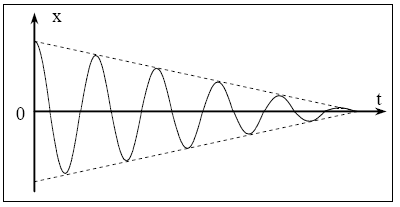
Oscillations amorties

L'amplitude $\mathrm{x}_{\mathrm{m}}$ diminue au cours du temps à cause des frottements et le mouvement finit par s'arrêter.

Oscillations avec des frottements fluides

(l'oscillateur est en contact avec un fluide)

a) Faible amortissement : régime pseudo-périodique. Plus l'amortissement est faible plus la pseudo-période est proche de la période-propre $T \approx T_0$.

b) Pour des frottements importants, l'oscillateur peut revenir à sa position de repos sans osciller : régime apériodique.

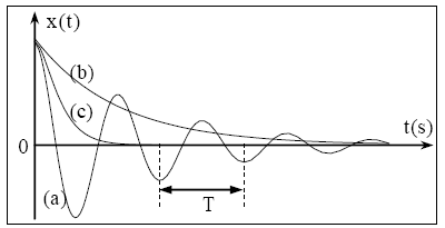
c) Pour une valeur particulière de la force de frottement, l'oscillateur retourne à sa position de repos, sans osciller, au cours d'une durée minimale : régime critique.
Cette situation est recherchée dans le cas des suspensions d'automobile.

Oscillations avec des frottements solides

(l'oscillateur est en contact avec un solide). Dans ce cas $\mathrm{x}_{\mathrm{m}}$ décroit linéairement au cours du temps.

Pendule de torsion